Deep Learning for Protein Annotation

Note: This article explains the paper Using deep learning to annotate the protein universe and is based on a presentation prepared for the course “Machine Learning for Biotechnology”.

Why Deep Learning in Biology

Deep Learning Explanation

In machine learning, we generally work with a labeled dataset with many features that serve as inputs to the models.

Source

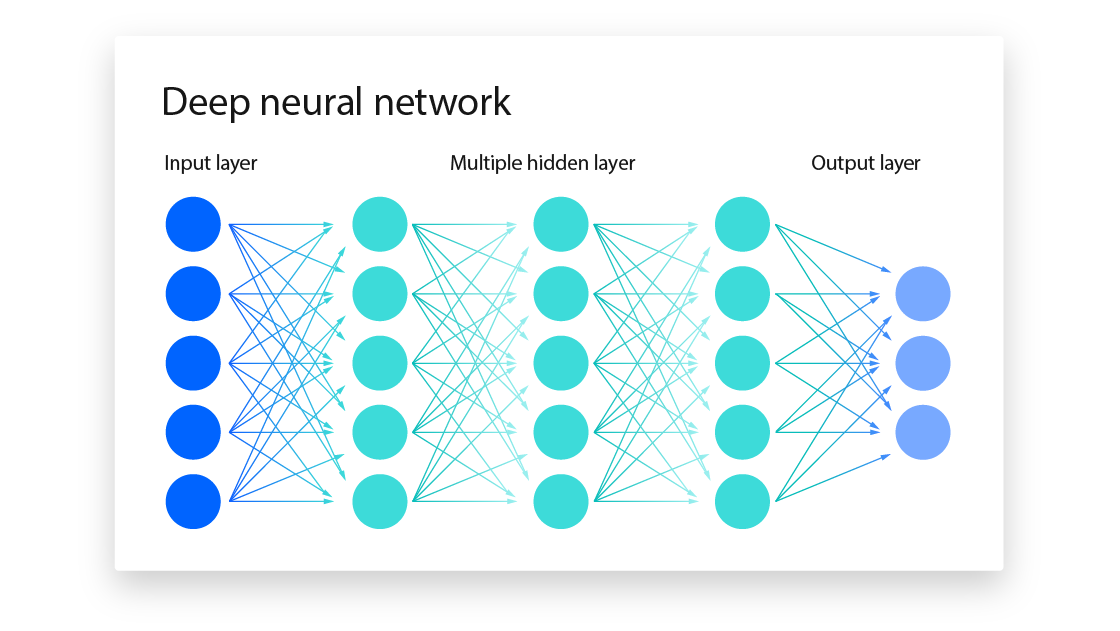
In deep learning, the input can be raw data instead of explicitly defined features. Deep learning benefits from neural networks that can understand the non-linear, complex relationships within the data—such as recognizing handwritten numbers in an image.

To recognize handwritten numbers, we feed the image into the input layer (on the left side) and obtain a final output (a digit from 0 to 9) at the output layer.

Source

Deep Learning Foundation: Large Labeled Datasets

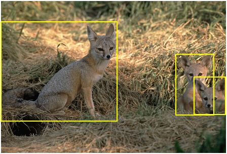
In the history of computer vision, a turning point was the creation of ImageNet, a dataset containing a large number of photos and annotations (e.g., in the image below, “foxes”).

Source

This dataset laid a solid foundation for the development of computer vision. Based on this dataset, computer scientists developed machine learning models that accurately predict the annotations of images.

In this process, many deep learning models emerged as scientists sought to better understand images, including the model we will explain later: the convolutional neural network. For instance, AlexNet, a CNN-based model, first emerged in 2012 and outperformed previous models.

Source

Biology: Rich in Labeled Datasets

Training deep learning models requires large amounts of high-quality labeled data. The founder of ImageNet, Fei-Fei Li, leveraged the power of crowdsourcing to label over 1,034,908 images with annotations.

Biology is also a rich source of large, high-quality datasets—for example, the sequences of proteins.

Source

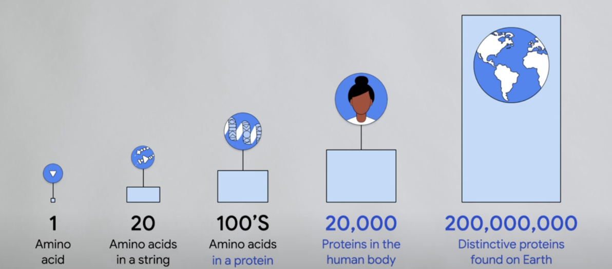
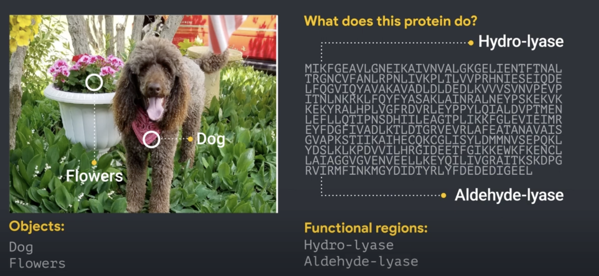
Just as machines are trained to understand objects in images, researchers aim to train machines to understand how amino acids influence a protein’s 3D structure and function:

Source

Note: For those who need a refresher on protein sequences: proteins are composed of chains of amino acids, and there are 20 different types. The unique combinations—varying in length and order—determine both the shape and function of each protein. For example, specific arrangements of amino acids enable us to have hair and muscle—both composed of protein, yet with completely different functions.

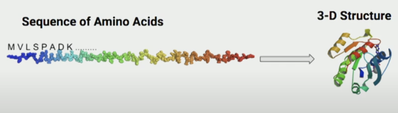
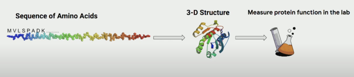
Deep Learning in Protein Sequence: 3D Structure and Function

In 2024, researchers at DeepMind won the Nobel Prize in Chemistry for solving a challenge that had stumped biologists for many years: given the sequence of a protein, what does it look like in 3D?

AlphaFold used deep learning models to predict the 3D structure of proteins and saved biologists significant time. For example, if a biologist wants to design a protein with a specific structure (to better interact with other molecules), instead of trying many combinations of sequences and testing each one experimentally, they can now use AlphaFold to iterate through the process.

Source

🧬 Side note: This video provides a nice introduction to how AlphaFold was developed and used for 3D structure prediction.

In this article, we will explore another deep learning model that addresses a different question: when we have the sequence of a protein, what is its function?

Source

From the Sequence to the Function: Sequence Alignment

Before deep learning models were used to annotate protein function, how did biologists do it?

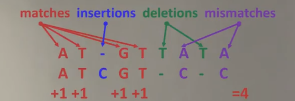
There is a method called sequence alignment. According to evolutionary theory, if two sequences share similarities, they likely have a common ancestor and possibly similar functions.

This approach is useful for biologists. Imagine someone discovers a new protein sequence—without performing further experiments, they can compare it to a database to see if it shares a similar structure with known proteins. This comparison provides a basic understanding of the new sequence.

Let’s use a simplified example to illustrate the concept:

Suppose we have two protein sequences: the first is ATGTTAT, and the second is ATCGTCC. We’d like to assess how well they align.

Using a simple scoring method, we might find a maximum score of 4, based on how many amino acids match and where insertions, deletions, or mismatches occur.

Source

Of course, in the real world, sequence alignment techniques are more complex than simply summing match scores. There are well-known tools like profile hidden Markov models (PHMMs) and BLASTp that can align sequences with high precision.

Source

However, even these advanced techniques have limitations—for instance, they could not annotate the function for one-third of known protein sequences. This is why a new technique—deep learning—was introduced.

Understanding the Data Source: Pfam

Just as the success of ImageNet was built on large-scale, human-labeled images, to predict the function of protein sequences we first need a reliable dataset.

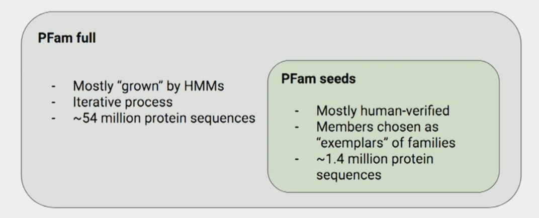
In this research, scientists used Pfam, a database of protein families with functional annotations.

There are two datasets:

• PfamSeed: Contains 1.4 million protein sequences, most of which are human-verified—making them more reliable.
• Pfam Full: Contains 54 million sequences, expanded mostly using sequence alignment techniques like HMMs.

Source

Let’s take a look at the PfamSeed dataset:

Source

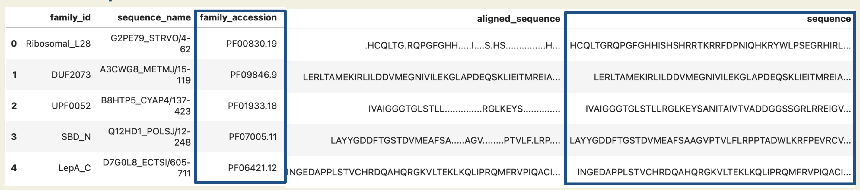
Each Pfam family_accession is associated with specific functions, so once the model can predict which family a protein sequence belongs to, it can also provide insights into that protein’s function.

Taking PfamSeed as an example, the researchers train the model on this dataset and predict the 1.4 million protein sequences into 17,929 families.

Understanding the Deep Learning Model: ProtCNN, ProtENN

There are two main deep learning models mentioned:

1. ProtCNN – a convolutional neural network (CNN)
2. ProtENN – an ensemble of 19 ProtCNN models

We’ll start by exploring ProtCNN.

ProtCNN Model Overview

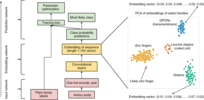
Below is the overall architecture of ProtCNN, as described in the paper. We will explain it layer by layer from bottom to top.

Source

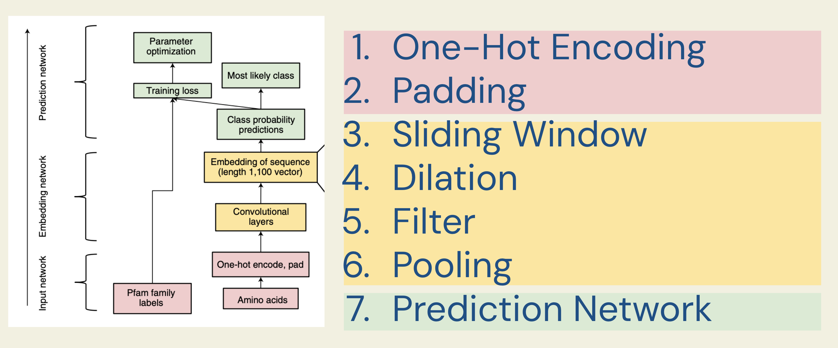
There are three major components in this model:

1. Input network: Processes protein sequences into a representation that machines can understand.
2. Embedding network: Learns hidden patterns in the sequence.
3. Prediction network: Uses these learned patterns to assign a function to the protein sequence.

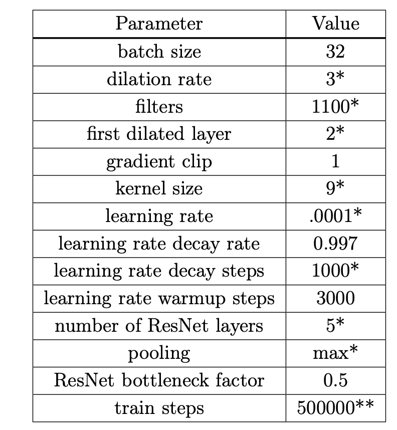
Many hyperparameters are used in this model; after extensive tuning (see the supplementary material for the search range), the following are used for the PfamSeed dataset, which we will refer to as we explain the CNN model:

Source

Input Network

A key idea in deep learning is breaking large computations into smaller tasks to leverage GPU parallelism. When handling a huge number of protein sequences, we need to preprocess them efficiently.

One-Hot Encoding to 1D Data: Vector

Just as machines understand images by converting them into numerical pixels, we convert protein sequences into numbers.
For example, consider the amino acid “A”. We convert it using one-hot encoding:

A: [1, 0, 0, 0, 0, 0, 0, 0, 0, 0, 0, 0, 0, 0, 0, 0, 0, 0, 0, 0]

Similarly, for “D”:

D: [0, 0, 1, 0, 0, 0, 0, 0, 0, 0, 0, 0, 0, 0, 0, 0, 0, 0, 0, 0]

The vector length is 20 because there are 20 types of amino acids.

Padding to a Fixed Length, 2D Data: Matrix

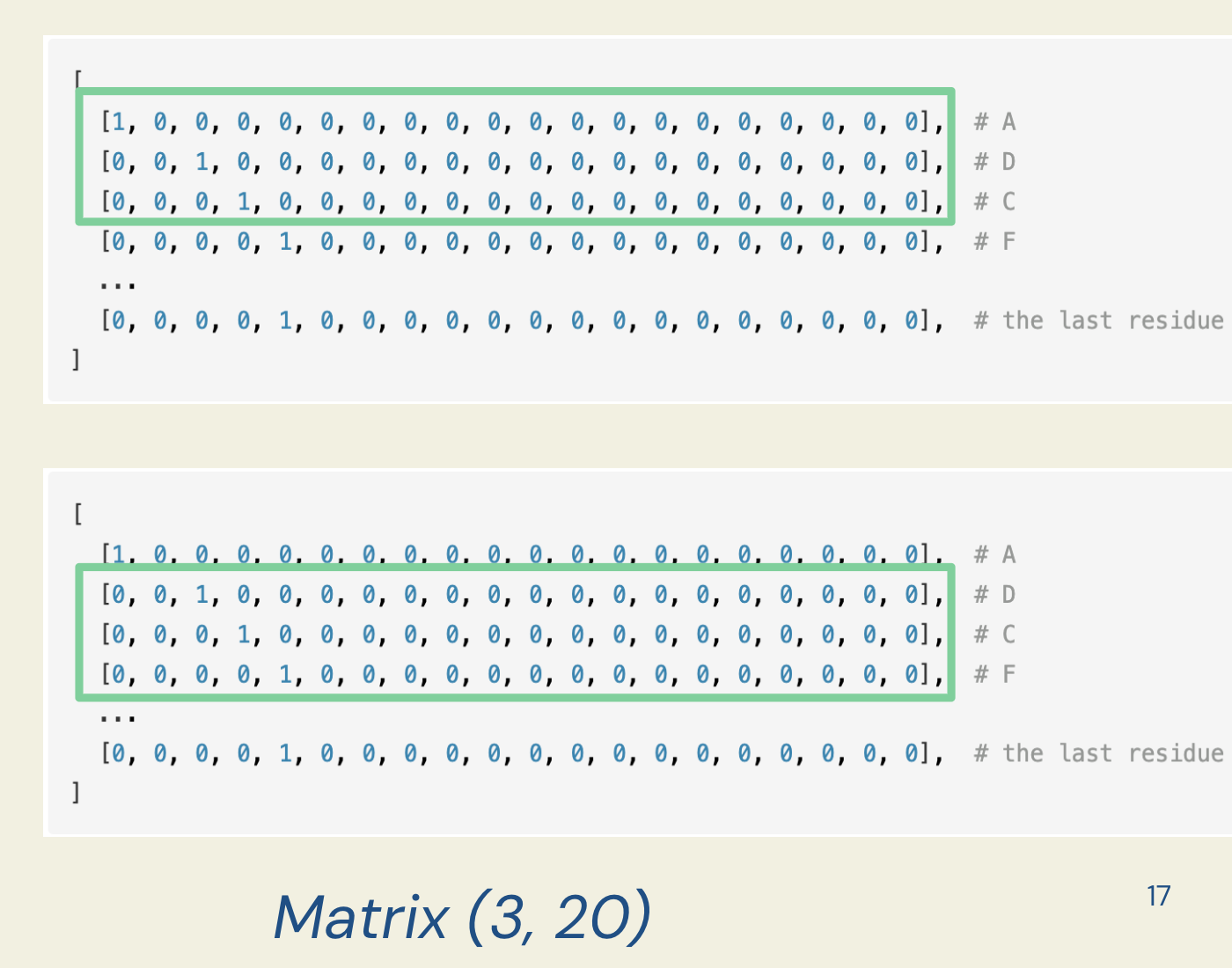
Now, if the sequence contains multiple amino acids—say ADC—we convert it into a 2D array (a matrix):

[
  [1, 0, 0, 0, 0, 0, 0, 0, 0, 0, 0, 0, 0, 0, 0, 0, 0, 0, 0, 0],  # A
  [0, 0, 1, 0, 0, 0, 0, 0, 0, 0, 0, 0, 0, 0, 0, 0, 0, 0, 0, 0],  # D
  [0, 1, 0, 0, 0, 0, 0, 0, 0, 0, 0, 0, 0, 0, 0, 0, 0, 0, 0, 0]  # C
]

Each row is a one-hot vector for a single amino acid.

However, protein sequences can vary in length, which is problematic for many models.

How do we preprocess sequences of different lengths?

Sequences are padded to the length of the longest sequence within each batch. If a sequence has fewer amino acids than the longest sequence in the batch, the remaining positions are padded with zeros.

Examining the sequence length distribution in the PfamSeed dataset reveals that most sequences are less than 1000, and there is a noticeable spike around 1100.

Source

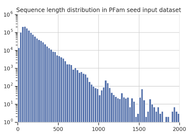
So, for illustration, we set a maximum sequence length of 1100 in the following examples. For any protein with fewer than 1100 amino acids, the remaining positions are filled with zero vectors.

For example, the sequence ADCC will change in shape from (4, 20) to (1100, 20)—with the remaining 1096 positions padded with zeros.

[
  [1, 0, 0, 0, 0, 0, 0, 0, 0, 0, 0, 0, 0, 0, 0, 0, 0, 0, 0, 0],  # A
  [0, 0, 1, 0, 0, 0, 0, 0, 0, 0, 0, 0, 0, 0, 0, 0, 0, 0, 0, 0],  # D
  [0, 1, 0, 0, 0, 0, 0, 0, 0, 0, 0, 0, 0, 0, 0, 0, 0, 0, 0, 0],  # C
  [0, 1, 0, 0, 0, 0, 0, 0, 0, 0, 0, 0, 0, 0, 0, 0, 0, 0, 0, 0],  # C
  ....
  [0, 0, 0, 0, 0, 0, 0, 0, 0, 0, 0, 0, 0, 0, 0, 0, 0, 0, 0, 0]  # Padding
]

3D Data: Tensor

Deep learning models process data in batches. In this research, the batch size is 32, meaning 32 protein sequences are processed simultaneously.

Thus, the data shape becomes:
(32, 1100, 20) = (batch size, sequence length, channels).

This creates a 3D array, called a tensor. Now, the input data is ready for the next step: the embedding network.

Embedding Network

The main goal for this step is to extract meaningful features from the raw data.

Sliding Window in CNNs

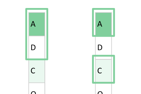
In CNNs, we use sliding windows to scan the input and extract local features.

For example, consider a protein sequence and a window size of 3 with a stride of 1 (meaning we move one amino acid at a time).

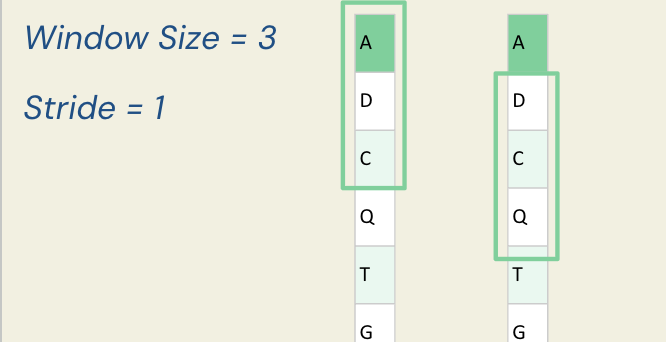
For the first window, we have ADC; for the second, we have DCQ.

Since we have already converted the sequence to a matrix via one-hot encoding, each sliding window corresponds to a 3×20 matrix.

Dilation

The main goal of dilation is to expand the input region (or,receptive field of the input, we will explain later) without increasing the number of parameters. With a single sliding window, we can capture features from more positions in the input.

For example, if we use a window size of 2 and no dilation, we select two nearby amino acids. However, if we introduce a dilation rate of 2, the model can “see” three amino acids and still select two of them—just with a “hole” between them.

In this paper, instead of using a fixed window size, the researchers use a window size of 9 and a dilation rate of 3 to better capture patterns in the data.

To understand dilation, consider the following illustration:

Source

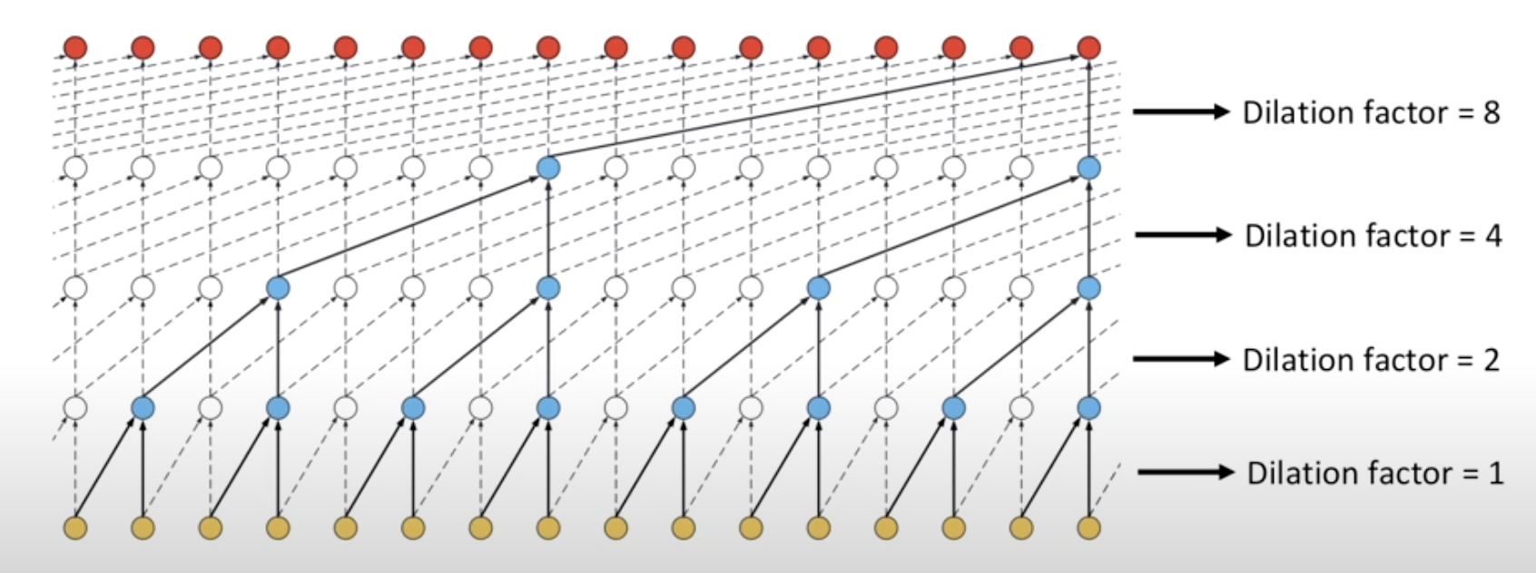
Dilation expands the effective input range by introducing “holes” into the convolution window. That is, the window still selects 9 positions, but these positions are spread out over a longer range in the sequence.

For each position in the sequence, the sliding window spans 25 positions in total. The formula is:

(kernel size - 1) * dilation + 1 = (9 - 1) * 3 + 1 = 25

From these 25 positions, 9 spaced-out amino acids are selected.

For example, at position 1, the selected positions are:

• Position 1
• Position 4 (1 + 3)
• Position 7 (4 + 3)
• Position 10 (7 + 3)
• Position 13 (10 + 3)
• Position 16 (13 + 3)
• Position 19 (16 + 3)
• Position 22 (19 + 3)
• Position 25 (22 + 3)

Each selected position has a one-hot encoded amino acid (a 20-dimensional vector).

[1, 0, 0, ..., 0]  # Position 1  
[0, 0, 1, ..., 0]  # Position 4  
...  
[0, 1, 0, ..., 0]  # Position 25  

Thus, the full sliding window consists of 9 amino acids × 20 dimensions, which is then flattened into a 1D vector of 180 numbers.

Layer by Layer

According to the paper, the first layer is non-dilated, and the following 5 layers are dilated with a fixed dilation rate of 3.

For the first dilated layer, the receptive field (the range of input positions a neuron can “see”) is 25 positions. For subsequent dilated layers, each adds an extra 24 positions to the receptive field. Therefore, we can calculate:

• Layer 1 (non-dilated): RF = 9.
• Layer 2 (dilated): RF = 9 + 24 = 33.
• Layer 3 (dilated): RF = 33 + 24 = 57.
• Layer 4 (dilated): RF = 57 + 24 = 81.
• Layer 5 (dilated): RF = 81 + 24 = 105.
• Layer 6 (dilated): RF = 105 + 24 = 129.

In other words, in the final layer, each residue’s feature incorporates information from up to 129 positions in the original protein sequence. The supplementary material includes a diagram that corresponds to this receptive field calculation:

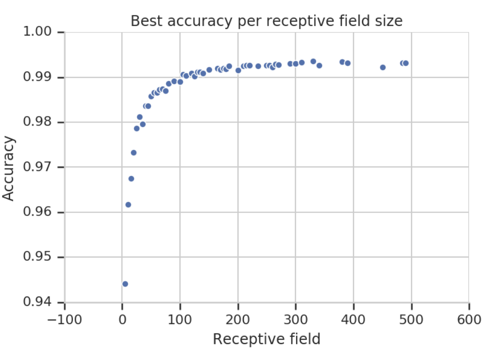
Once the receptive field exceeds a certain threshold (in this case, around 100 residues), further increases in receptive field size (e.g., from 100 to 500) do not significantly improve accuracy.

Filters

For each sliding window that captures local features, we want to detect whether it matches a certain pattern. In CNNs, these are implemented as filters (or kernels).

For example, in image detection, one filter might detect edges while another might sharpen the image:

Source

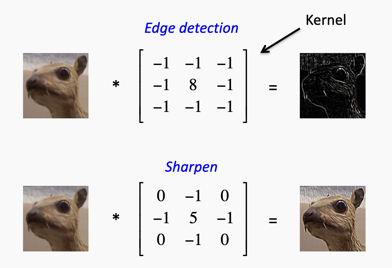
The filter weights are learned (along with a bias) and vary across layers during the traning. For instance, one filter might eventually learn to detect a particular protein motif associated with a specific function.

Suppose Filter 1 has weights: [0.1, 0.2, ..., 0.4, 0.5] (length = 180) and a bias of 0.05. When applying the filter, we compute the dot product between the filter and the 180-dimensional input vector:

(1 * 0.1) + (0 * 0.2) + ... + (1 * 0.5) = 0.6  
0.6 + 0.05 (bias) = 0.65

This value (0.65) indicates how strongly the feature is present in that window. A higher value means the feature is more prominent, similar to detecting a stroke in a handwritten digit.

For each sequence position, this operation is repeated across 1100 filters. So for position 1, you obtain a 1100-dimensional vector such as: [0.65, -0.10, ..., 1.22, 0.37] Repeating for all 1100 positions results in a matrix of shape (1100, 1100).

Thus, the tensor shape changes to:
(batch size, sequence length, filters) = (32, 1100, 1100)

Pooling

To further aggregate the information before final prediction, max pooling is applied.

Here’s an example: if we use a 2x2 window on the feature map and take the max number from each section, the method is called max pooling and it cam intensify key features in the feature map.

Source

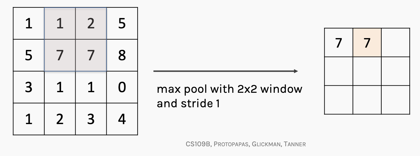
In the ProtCNN model, global max pooling is applied along the sequence dimension (over 1100 filters).

As explained earlier, for each position we have a vector of 1100 values (the responses from 1100 filters). The global max pooling operation selects the highest value for each filter across all positions, reducing the shape to: (32, 1100, 1) , which preserves the strongest signal per filter over the entire sequence.

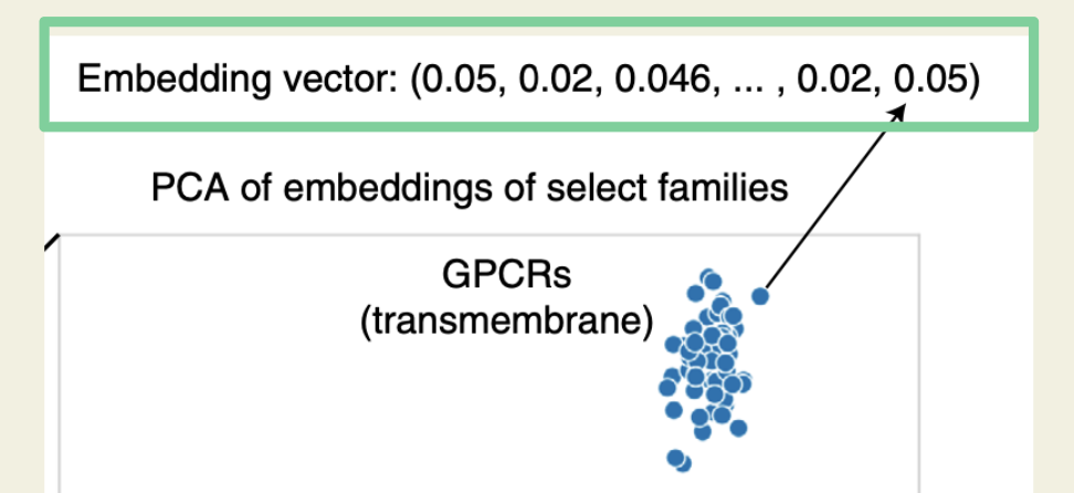
In other words, for each protein sequence, the final embedding is a 1×1100 feature vector. When applying PCA on these embeddings, protein sequences with similar functions tend to group together.

Prediction Network

Once we have the embedding (the learned representation of the sequence), it is fed into the prediction network and return us with the protein family label.

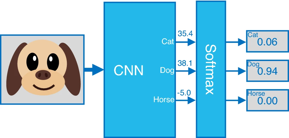
Analogy in Image Classification

For example, in image classification with three possible labels, the output of the fully connected layer is a three-dimensional vector containing the raw scores for each label. In the example image below, the raw score for the class labeled “dog” is 38.1.

Subsequently, the raw scores are passed through a SoftMax activation function, which converts them into a probability distribution over the possible labels. For instance, the output is also a three-dimensional vector, but this time it represents probability scores. The probability for the class labeled “dog” is 0.94.

Source

In the ProtCNN Model

In the fully connected layer, each protein sequence is transformed into a 17,929-dimensional vector of raw scores—one for each protein family.

After applying the SoftMax function, this 17,929-dimensional vector is converted into probabilities, representing the likelihood of the sequence belonging to each protein family.

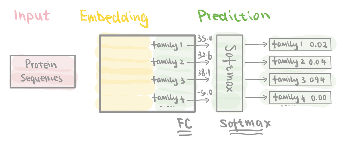
As each Pfam family corresponds to a known structural or functional group of proteins, classifying a sequence into one of these families also provides a prediction of the protein’s function.s, classifying a sequence into one of these protein families also predicts the protein’s function.

Bring It All Together: ProtENN

While ProtCNN is already powerful, it can benefit from model ensembling. That’s where ProtENN (Ensemble Neural Network) comes in—it combines 19 ProtCNN models into an ensemble.

These 19 ProtCNN models share the same architecture but are initialized with different random weights and trained independently on the same dataset.

The final ProtENN aggregates the predictions (or logits) from each model using majority voting, which helps reduce the overall error rate.

ProtREP

ProtCNN and ProtENN perform well, but they can struggle with very small families—families that have only a few training examples. This is where methods like ProtREP and other recent approaches come into play.

Note: Due to time constraints, this paper does not delved into the advanced ResNet/CNN details, the inner workings of ProtREP, or the amino‑acid embedding analysis; these topics may appear in future editions.

Results: ProtENN in Pfam

With the model defined, this section discusses how it trains and performs on annotating protein families in Pfam.

Dataset Splits

Like in all machine learning work, we need to split datasets into training, dev, and test sets. The model is first trained on the training dataset, and by examining the test set, we evaluate the model’s accuracy.

The key here: we want the training and test datasets to share similarities so that we can generalize the model to other data, but we don’t want them to be too similar, as that may cause overfitting.

The paper mainly discusses two ways of splitting the dataset:

1. Random Split: Randomly splitting the Pfam dataset results in training data that are similar to the test data.
2. Clustered Split: Grouping protein sequences based on similarities ensures that test data do not contain similar protein sequences.
   • This split is more challenging for deep learning as it requires capturing features that lie beyond simple sequence similarity, also known as remote homologues.

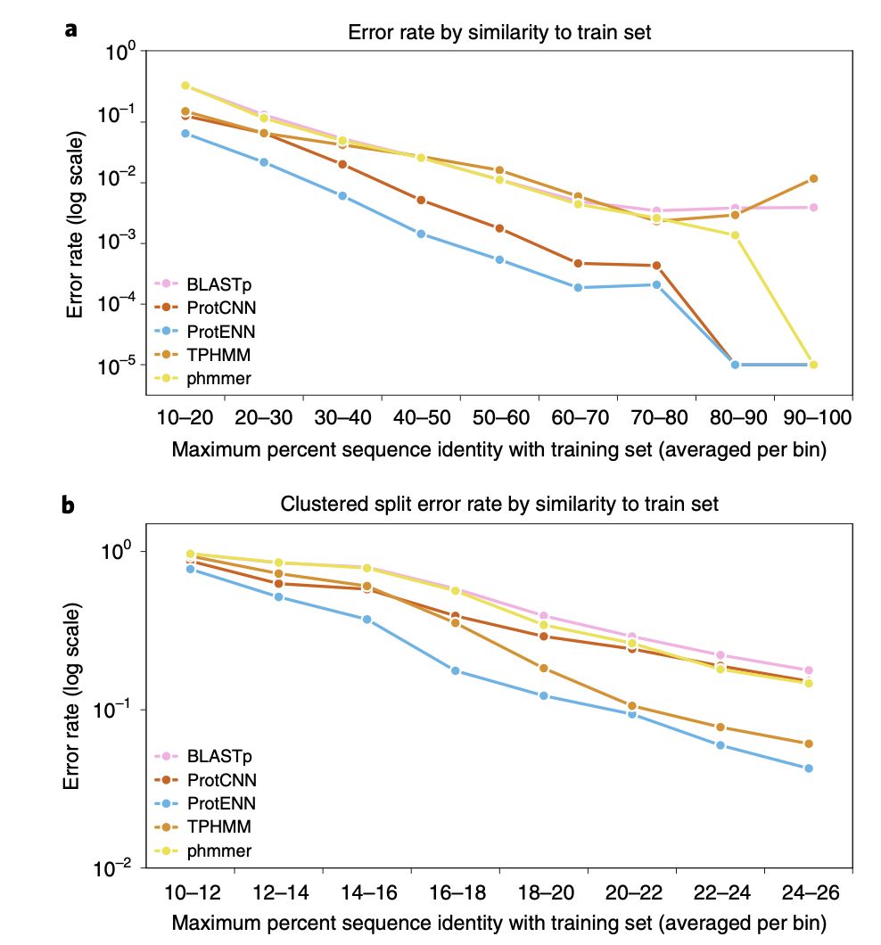
The paper mentions that, for both methods, ProtENN outperforms other models. The figures used in the paper are primarily based on the clustered datasets, which we will explore further in the following section.

Positive Outcome

Alignment-based techniques (e.g., TPHMM) and deep learning models can complement each other. For example, combining them improved accuracy of remote homology sequence classification from 89.0% to 93.3%.

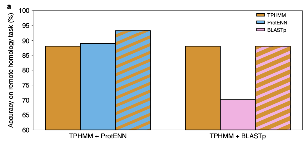
In detail:

• If HMMER is highly confident (e.g., it reports a low E-value), its prediction is used.
• Otherwise, the system falls back on the ProtENN prediction.

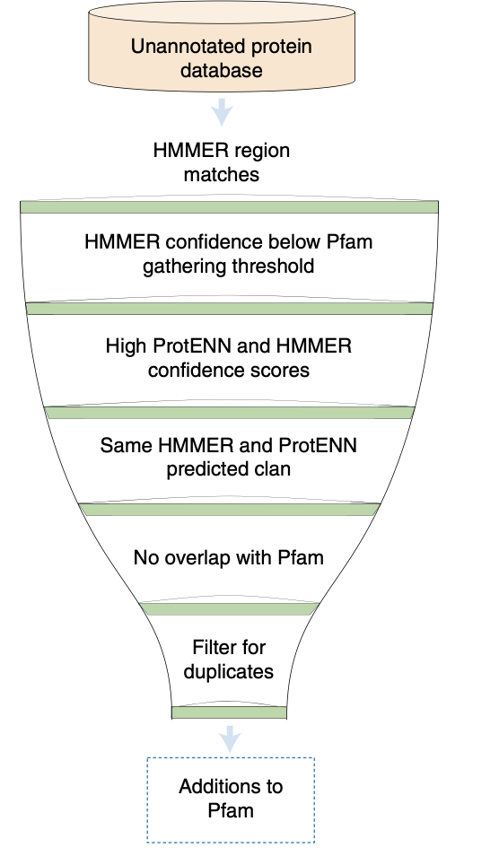
After training on Pfam-Full, the model was applied to approximately 140 million unannotated regions, increasing Pfam coverage by about 9.5%—this corresponds to 6.8 million new domain annotations, which exceeds the number of annotations added over the last decade.

They named this expanded annotation set Pfam-N, released as part of Pfam 34.0.

Further Research: Predicting Protein Function from Sequence

Since the paper’s publication in 2022, researchers have continued to push forward.

Large Language Models

For example, researchers have explored treating protein sequences like natural language by using large language models (LLMs) to understand them.

Instead of directly predicting function labels, ProtNLM generates natural language descriptions, similar to descriptions in databases like UniProt and InterPro. These descriptions help biologists understand protein functions more intuitvely.

Source

However, LLMs can sometimes “hallucinate,” so a method called retrieval-augmented generation (RAG) has attracted attention. This approach feeds the LLM real, reliable domain-specific data before asking for predictions.

In the case of protein function, instead of relying solely on the model’s training, we first retrieve relevant annotated protein sequences (e.g., using BLAST), and then feed those into the LLM along with the query. This approach is used in a recent method called ProtEx.

Source

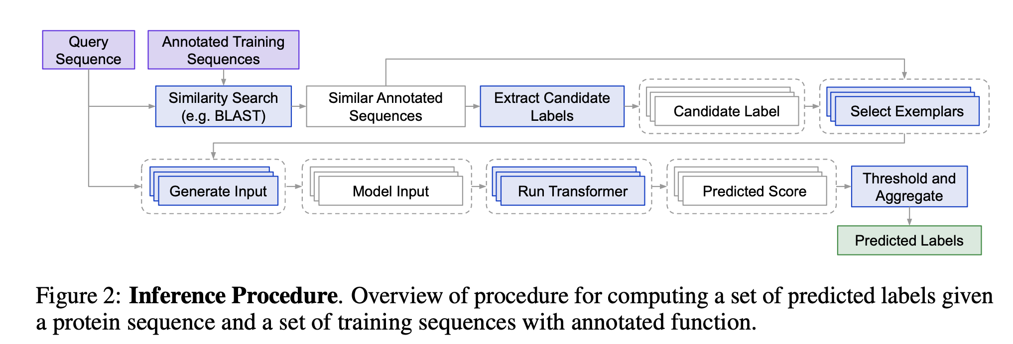
ProtEx retrieves real, high-confidence annotated examples (i.e., exemplar sequences) through BLASTp, then combines them with the query and label as input for the transformer model.

Want to Know More?

The following resources have helped me better understand this topic. Feel free to explore them if you’re curious too:

📄 On This Paper

• Main paper: Using deep learning to annotate the protein universe
• Supplementary materials: PDF - Supplementary Materials
• Code demo (step-by-step ProtCNN build):
  Google Colab Notebook
• Talks from the authors:
  • Podcast with first author Maxwell L. Bileschi
  • Conference talk by second author David Belanger

🤖 On Deep Learning (mainly on CNNs)

1. Harvard CS109B Course Materials
   • Especially Lecture 8 slides and Lecture 9 slides
2. VU University Amsterdam Deep Learning Course Materials
   • Especially the 1D convolution data explained
3. Interactive tools to better understand CNNs:
   • Handwritten number detection visualization
   • Image detection visualization
4. Understanding the Convolutional Filter Operation in CNNs